BRB-seq pipeline – downstream analysis best practices

In this post, we will see briefly how to perform downstream analysis for RNA-seq data.

The only difference is that we can run all downstream analyses on the raw read count matrix, or the UMI-deduplicated count matrix.

Standard analysis pipelines are scripted in R or in Python. In this post we will mainly use R because it’s the accepted standard for RNA-seq analyses, but similar analyses and results can be obtained using Python. First, the data needs to be loaded from the file into the R environment, using base commands such as read.table, or more advanced (faster) ones, such as fread (from the data.table package).

# Reading the transcriptomics data
library(data.table)
data.raw <- fread("my_count_matrix.txt", sep="\t", header = T, data.table = F)
rownames(data.raw) <- data.raw[,1]
data.raw <- data.raw[,-1]

Of note, here we use the tabulation as separator, and suppose that the count matrix has a header (with the sample names), and that the first column contains gene names (or identifiers).

Finally, we remove the first column containing the gene names. Of course, this is to be repeated if you need to load external metadata, for example for loading groups, covariates, or other phenotypes.

# Compute depth per sample
data.meta <- data.frame(samples =ccolnames(data.raw), depth = colSums(data.raw))
# Filter samples that did not aggregate at least 1M reads
outliers <- subset(data.meta, depth < 1E6)$samples
data.raw <- data.raw[,-which(colnames(data.raw) %in% outliers)]
# Filter low expressed genes
data.raw <- data.raw[rowSums(data.raw > 1) > 4,] # At least 1 read in 4 samples

Once the data is filtered, it should be normalized. In particular to remove the effect of sequencing depth and thus be able to compare the samples on a similar depth basis.

# Normalization using limma-voom
library(limma)
data.norm <- voom(counts = data.raw, normalize.method="quantile")$E

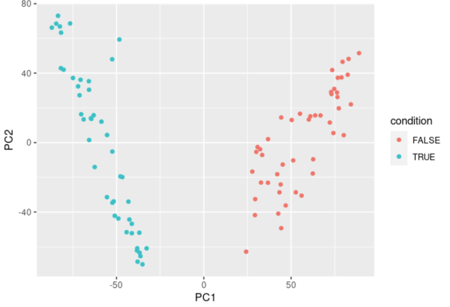
Then, at this stage, we usually want to visualize our data. We can do this using dimension reduction methods such as Principal Component Analysis (PCA) or MultiDimensional Scaling (MDS).

# PCA
data.pca <- data.frame(prcomp(t(data.norm), center = T, scale. = T)$x)

# Plot
library(ggplot2)
ggplot(data.pca, aes(x = PC1, y = PC2)) + geom_point()

  

# Importing the biological effect     studied (from a metadata file, or manually, or…)
data.condition <- c(T, T, T, T, …, F, F, F, F) # Binary     condition here

# Plotting the PCA with coloring by     condition
data.pca$condition <- data.condition
ggplot(data.pca, aes(x = PC1, y = PC2, col = condition)) + geom_point()

Now, the goal is often to find Differentially Expressed (DE) genes between your two conditions. Again, there are many methods for doing as such (limma, DESeq2, edgeR, …). We used limma-voom for normalizing, so that makes sense to run limma for DE.

# Remove genes without variance
data.norm <-     data.frame(data.norm[which(apply(data.norm, 1, var) != 0),])

# Create the design matrix based on     your condition
# Of note : Here you can add     covariates to the model (batch, sex, …) if you have in your data that may     bias the signal of your biological condition
data.design <- model.matrix(~data.condition)

# Run the DE model
fit <- lmFit(data.norm, data.design)
fit <- eBayes(fit)

# Create the table with     all DE results
DE.table <- topTable(fit, n=Inf, adjust="fdr",     sort.by = "none") 

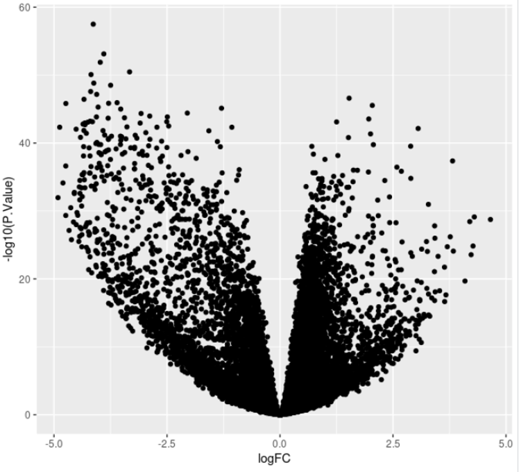
# Volcano plot
ggplot(DE, aes(x = logFC, y = -log10(P.Value))) + geom_point()

This will generate the following plot:

 

Now, we need to set some thresholds to select Differentially Expressed Genes (DEG). Usually, we set a threshold on the statistical significance (adjusted p-value, FDR) and one on the effect size of the change (fold-change).

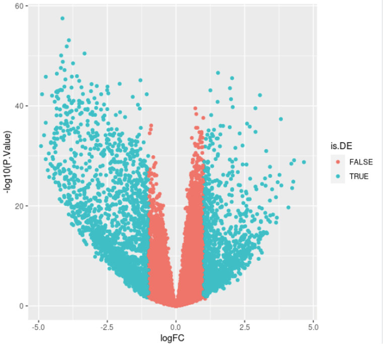
# Filter results (Here FDR <= 5%     and FC > 2)
DE$is.DE <- DE$adj.P.Val <= 0.05 & abs(DE$logFC) > log2(2)
# Volcano plot
ggplot(DE, aes(x = logFC, y = -log10(P.Value), col = is.DE)) +     geom_point()
# Filter the DE table
DE <- subset(DE, is.DE)
message(nrow(DE), " DE genes found: ", sum(DE$logFC > 0),     " up-regulated, and ", sum(DE$logFC < 0), " down-regulated")

Which messages something like: "3344 DE genes found: 1326 up-regulated, and 2018 down-regulated" and plots the following: 

 

Of course, the sign of the fold-change depends on which group you took as “reference”, so the number of up- or down-regulated genes can be inverted if the reference group changes.

 

# Sort the DE genes by effect size     (Fold Change)
# Top up-regulated
DE <- DE[with(DE,     order(-logFC)),]
top_20_up_genes <- rownames(DE)[1:20] # Keeping the top up-regulated     genes for later
fwrite(x = DE, file = "DE.genes.txt", sep = "\t",     quote = F, row.names = T, col.names = T)
# Or alternatively, sort     by putting the down-regulated genes at the top
DE <- DE[with(DE, order(logFC)),]
top_20_down_genes <- rownames(DE)[1:20] # Keeping the top 20 down-regulated genes

You can then sort the DE table and save it as an external text file using write.table or fwrite

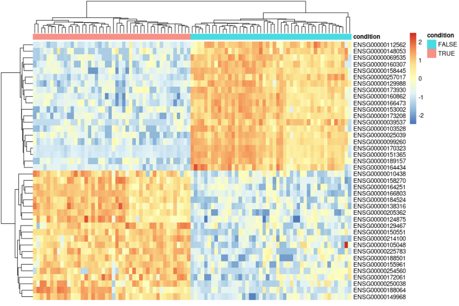
# Create a data.frame containing the     condition, for annotation of the heatmap
data.annotation <- data.frame(row.names = colnames(data.norm),     condition = factor(data.condition))
# Plot the heatmap
library(pheatmap)
pheatmap(data.norm[c(top_20_up_genes,top_20_down_genes),],     scale = "row", annotation_col =     data.annotation)

This will generate the following plot:

 

After that, the rest of the analysis consists of performing gene set enrichment, for e.g. using Gene Ontology terms, or KEGG pathways. This helps explaining the effect of the DE genes. Other possibilities are to focus on known genes and show that they are indeed differentially expressed. But this is mostly depending on the hypothesis that one is evaluating.

For more information about RNA-seq and BRB-seq data analysis do not hesitate to reach out at info@alitheagenomics.com